Permutations

An important object in discrete mathematics is called permutation - a bijective mapping between set $X$ and itself. From Theorem 24¹, there are a total of $n!$ permutations on a set $X$ of size $n$. For instance, when $X= \{1,2,3\}$, a bijective mapping $f$ can be defined as $f(1) = 2$, $f(2) = 1$, and $f(3) =3$.

We can write $f$ in a two-row representation:

$$\begin{pmatrix} 1 & 2 & 3\\ 2 & 1 & 3 \end{pmatrix}$$

The first row lists all elements of $X$ and, under each element $x \in X$, we list $f(x)$ right under it. In fact, we only need one line to represent such a permutation: Just take the second line $(2, 1, 3)$, which means that $f(1) = 2$, $f(2)=1$ and $f(3)=3$. Note that such a representation suffices since we know that the permuted items are listed under a fixed total order of $X$ (in this case the natural increasing order $1,2,3$).

Figure 11: A graphical representation of $(4, 8, 3, 5, 2, 9, 6, 1, 7)$.

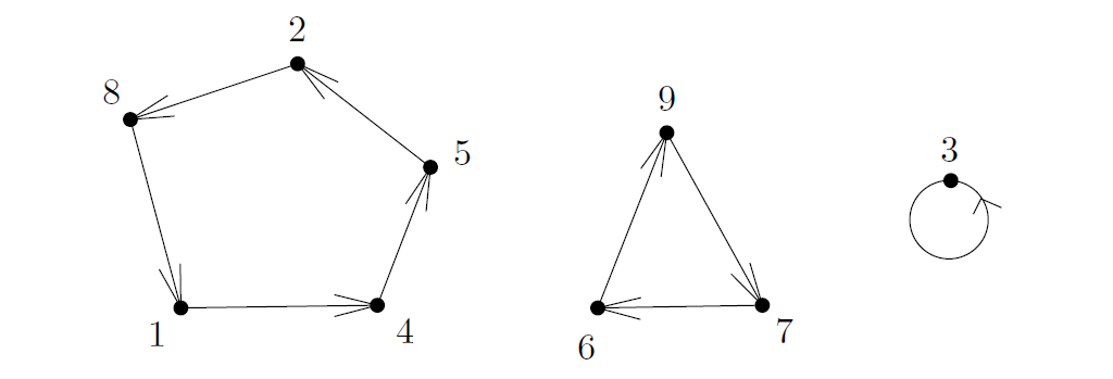
Figure 11 shows a graphic representation of permutations where an arrow from $i$ to $j$ represents $f(i) =j$. It is easy to see (by picture) that each permutation has a representation that is a union of disjoint cycles. Again, no matter how you try to draw a permutation, you will see this fact. So it is obvious in drawing, but how do we really define these cycles formally?

Example 23 (Composition of permutations)

Let $f$ and $g$ be two permutations on $X$. Define $f \circ g$ as $f\circ g(i) = f(g(i))$. Notice that $f\circ g$ is also a permutation on $X$.

Proof:

We need to argue one-to-one and onto properties. For the one-to-one, assume that $f\circ g(i) = f\circ g(j)$; so $f(g(i)) = f(g(j))$. Since $f$ is one-to-one, we have $g(i) = g(j)$; since $g$ is one-to-one, we have $i = j$. To show the onto property, consider $j \in X$. Since $f$ is onto, we have that there exists $x\in X$ for which $f(x) = j$; since $g$ is onto, there exists $y \in X$ for which $g(y) = x$; therefore, $f\circ g(y) = f(g(y)) = f(x) = j$.

For any permutation $f$, we define $f^k$ as the permutation that is a $k$-fold composition of $f$ with itself, i.e., $f^1 = f$ and $f^k = f\circ f^{k-1}$. Define the relation $\approx$ on the set $X$ where $i \approx j$ if and only if there exists $k \geq 1$ such that $f^k(i) = j$.

Exercise 61

Prove that $\approx$ is an equivalence relation and that its equivalence classes are the cycles of $f$.

Define the identity permutation ${\sf id}$ on $X$ as ${\sf id}(i) = i$ for all $i \in X$.

Exercise 62

Let $\pi$ be a permutation. Prove that there exists integer $k$ for which $\pi^k = {\sf id}$. As a bonus, describe an algorithm that, given a permutation $\pi$, computes the minimum value of $k$ satisfying the former property.

Derangements

Now we will consider an interesting example of counting that requires non-trivial, creative thinking. Suppose there are $n$ students in class, and we (teachers) already graded the student's homework. If we shuffle the graded homework at random before returning them to students, how many students should we expect to receive their own homework? This is a non-trivial question, and we will see several ways to answer this question.

We say that a permutation $\pi$ on $[n] = \{1,\ldots, n\}$² is a derangement if $\pi(i) \neq i$ for all $i \in [n]$. In other words, $\pi$ does not have a fixed point.

The question here is, out of the $n!$ permutations, how many of them are derangements?

Let $\Pi_n$ be the set of derangements on $[n]$ and $D_n= |\Pi_n|$ be the number of such derangements. We will prove the following recurrence:

Theorem 25

$D_n = (n-1)(D_{n-1} + D_{n-2})$

Proof:

We want to count the number of derangements $f$ on $[n]$. First, notice that $f(n)$ can map to $(n-1)$ possibilities (anything but $n$). We partition the derangements in $\Pi_n$ into $(n-1)$ sets based on this value, i.e., $\Pi_{n,i} = \{f \in \Pi_n: f(n) = i\}$, so we have that $|\Pi_n| = \sum_{i=1}^{n-1} |\Pi_{n,i}|$. By a bijection argument, it is easy to see that the sets $\Pi_{n,i}$ are of equal size, so we have that $|\Pi_n| = (n-1)|\Pi_{n, n-1}|$.

For simplicity, denote $\Pi_{n,n-1}$ by $\mathcal{F}$. We further partition $\mathcal{F}$ into $\mathcal{F}_1$ and $\mathcal{F}_2$ based on the value of $f(n-1)$:

$\mathcal{F}_1 = \{f \in \mathcal{F}: f(n-1) \neq n\} \text{ and } \mathcal{F}_2 = \{f \in \mathcal{F}: f(n-1) = n\}$

The key observations are that: (i) there is a bijection between $\mathcal{F}_1$ and $\Pi_{n-1}$ (this is very easy to see) and (ii) a bijection between $\mathcal{F}_2$ and $\Pi_{n-2}$. In the exercises, you will formally prove these.

Exercise 63

Formally complete the proof of the above theorem. In particular,

• describe a bijection between $\Pi_{n,n-1}$ and $\Pi_{n,i}$ for all $i\in[n-1]$,
• describe a bijection between $\mathcal{F}_1$ and $\Pi_{n-1}$, and
• describe a bijection between $\mathcal{F}_2$ and $\Pi_{n-2}$.

We want to remark that the above theorem immediately implies a computational solution for the number of derangements. With the recurrence relation, it is relatively straightforward to code a dynamic programming (DP).

Exercise 64

Derive the following explicit formula for $D_n$:

$D_n = n! \sum_{k=0}^n \frac{(-1)^k}{k!}$

Hint: Define $C_n = D_n - n \cdot D_{n-1}$. Write the recurrence for $C_n$ and solve it.

Mathematical theory of sorting

In computer science, we encounter permutations very often, most notably in the context of sorting. In this section, we will treat sorting as a purely mathematical topic. A sorting algorithm $A$ can be seen as a mapping that takes a permutation $\pi: [n] \rightarrow [n]$ as input and performs a sequence of exchange operations until $\pi$ becomes an identity permutation ${\sf id}$. A good sorting algorithm is one that uses as small number of exchange operations as possible.

Figure 12: Composition of permutation $\pi= (2,1,5,3,4)$ with $g={\sf swap}_{3,5} = (1,2,5,4,3)$. The arrows on the left and right show the mapping of $g$ and $\pi$ respectively. The outcome of this composition is $\pi \circ g= (2,1,4,3,5)$ (obtained by swapping numbers in $\pi$ in the 3rd and 5th positions).

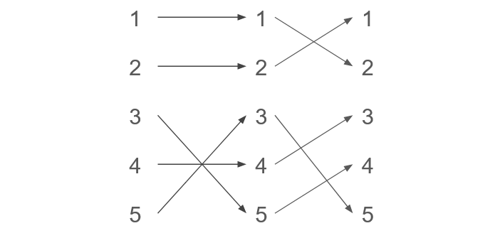
An exchange operation can be seen as composing the input permutation (the unsorted elements) with a swap permutation: ${\sf swap}_{i,j}(i) = j, {\sf swap}_{i,j}(j) = i$, and ${\sf swap}_{i,j}(k) = k$ for $k \not\in \{i,j\}$. Intuitively, if we represent a permutation $\pi$ in a one-line notation, applying the composition ${\sf swap}_{i,j}$ would exchange the numbers in the $i$-th and $j$-th position of the permutation. See Figure 12 for illustration. The following claim makes this discussion formal.

Proposition 2

If $\pi = (p_1,\ldots, p_n)$ and $1 \leq i<j\leq n$, then

$\pi \circ {\sf swap}_{i,j} = (p_1,\ldots, p_{i-1}, p_j, p_{i+1} \ldots, p_{j-1}, p_i, p_{j+1}, \ldots, p_n)$

Therefore, a sorting algorithm $A$ can be seen as, on input permutation $\pi$, output a collection of $\{(i_1,j_1),\ldots, (i_q, j_q)\}$ so that $\pi \circ {\sf swap}_{i_1, j_1} \circ {\sf swap}_{i_2,j_2} \cdots \circ {\sf swap}_{i_q, j_q} = {\sf id}$. For instance, to sort a permutation $\pi = (1,2,4,3)$, we can compose $\pi$ with $g = {\sf swap}_{3,4}$, and $\pi \circ g$ gives us an identity permutation.

Let $\pi$ be a permutation. We say that $(i,j)$ is an inversion of $\pi$ if $i <j$ and $\pi(i) > \pi(j)$. Denote by $I(\pi)$ the set of all inversions of $\pi$. This notion of inversion captures exactly the locations of $\pi$ that are currently in an "swapped" relative order and need to be "inverted" somehow. Notice that the identity ${\sf id}$ has $I({\sf id}) = \emptyset$, and the reverse permutation $(n,n-1,\ldots, 2,1)$ has $n(n-1)/2$ inversions. In this way, $I(\pi)$ measures how far $\pi$ is from an identity permutation.

Exercise 65

Prove that $I(\pi)$ is transitive (i.e., prove that if $(i,j)$ and $(j,k)$ are inversions, then so is $(i,k)$)

The concept of inversion can be used to analyze the performance of some natural sorting algorithms. In particular, we learn from algorithms classes that the best sorting algorithms take $O(n \log n)$ steps. However, if sorting algorithms are allowed to only exchange consecutive numbers, it is known to be unable to achieve the optimal performance.

Exercise 66

Consider a sorting algorithm $A$ that only exchanges two neighboring locations (i.e., performing ${\sf swap}_{i,i+1}$ for some $i$). Prove that there exists a permutation $\pi$ for which $A(\pi)$ must perform at least $\frac{n^2}{10}$ exchange operations.

Footnotes

1. Note that a one-to-one function is also "onto" if it maps objects from a finite set to itself. ↩

2. Note that here we redefined $[n]$ to start from one. This is usually more convenient when counting whereas starting from $0$ is usually more convenient when working with modulo operations as in Number and Algorithms. ↩